Amortised learning for generic generative models
A popular objective of unsupervised learning nowadays has been to achieve high log-likelihoods on MNIST digits and generating realistic sample images. We set out to follow that trend, but didn’t quite make it. Nonetheless, we discovered so much that I’d like to share in this post, including the algorithm of amortised learning by wake-sleep we proposed. This is a collaboration with Theodore Moskovitz, Heishiro Kanagawa and my supervisor Maneesh Sahani.
Acknowledgement
The core idea has been around in our lab for some time during the work on distributed distributional code by my supervisor Maneesh Sahani and fellow PhD (then student) Eszter Vértes. Dating way back, the wake-sleep component was born with the Helmholtz machine by Peter Dayan and Geoffrey Hinton when they were still around our lab.
The usual path of the ELBO
Many unsupervised learning algorithms rely on fitting generative models on datasets. We focus on a broad class of generative models that can be written as $p_\theta(z,x)=p_\theta(z)p_\theta(x|z)$ where $z$ denotes all latent variables, and $x$ denotes the observations. Note that this model could have any arbitrary graphical structure: the latent $z$ can be a tree, a Markov chain (giving hidden Markov models) or even loopy. Due to the intractable normaliser, we cannot compute the log-likelihood \(\log p_\theta (x) = \int p_\theta(z,x)\text{d}z\) or its gradient directly.
From textbooks, we know that an alternative objective is the ELBO or free energy
\[\mathcal{F}(q,\theta)=\mathbb{E}_{q(z)}[\log p_\theta(z,x)] + \mathbb{H}[q] \le \log p_\theta(x)\]where $q$ is some distribution over $z$ and $\mathbb{H}[q]$ is its entropy. We can optimise this lower bound w.r.t. $\theta$ and $q$ by the expectation-maximisation (EM) algorithm.
Since the optimal \(q\) obtained is almost always an approximate posterior, the gradient computed from the ELBO is biased from the true log-likelihood gradient. A (real) ton of work has been put on how to improve this $q$. As there is practically no way of computing the true posterior, the accuracy of an approximate inference scheme is usually measured indirectly by the quality of generative models they could train, using log-likelihoods, sample quality of other downstream tasks (thanks to diverse tasks a generative model affords).
As we shift towards amortised inference, more flexible and higher-dimensional generative model can be trained. When the generative model $p_\theta$ is defined with very flexible neural networks, inference becomes even more challenging. We show this in Figure 1 of our paper: after training a vanilla VAE with 2-dimensional $z$ on MNIST digits, the induced true posteriors can have very irregular shapes and even multiple modes. This is despite the simple Gaussian posterior distributions the generative model sees during training. Approximating these posteriors is just hard…
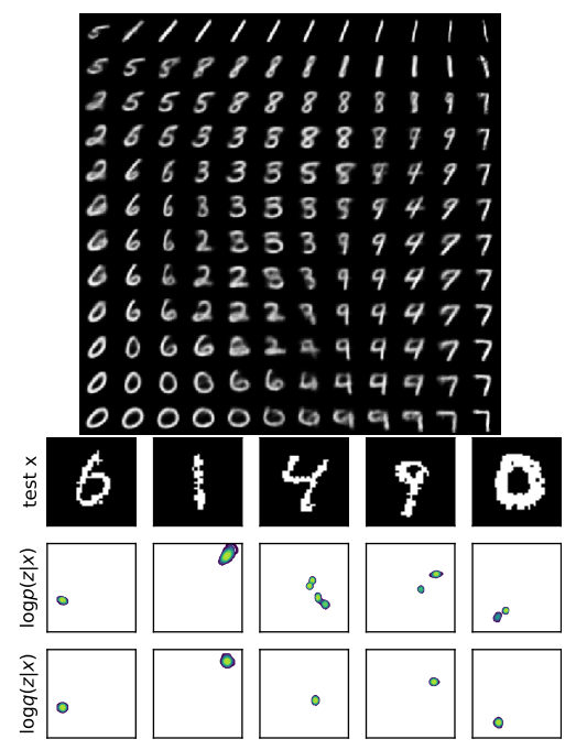
VAE trained on binarised MNIST digits. Top: mean images generated by decoding points on a grid of 2-D latent variables. Bottom three rows show five samples of real MNSIT digit (top), the corresponding true posteriors (middle) found by histogram and the approximate posteriors computed by the encoder.
The unusual path If we just care about learning $\theta$…
then is it really necessary to try and nail those weird posterior distributions? Maybe not…
Suppose we apply iterative updates to $\theta$ , and we are at $\theta_t$ for the $t$’th iteration. What do we do? Using EM, we would first compute an approximate posterior $q$ . The best $q(z)$ is the exact posterior $p_{\theta_t}(z\vert x)$ – see the $\theta_t$ in the subscript? The posterior is always for a fixed $\theta=\theta_t$ . A perhaps less intuitive property of the ELBO is:
\[\begin{equation} \nabla \mathcal{F}(p_{\theta_t}(z|x),\theta)\vert_{\theta_t}= \mathbb{E}_{p_{\theta_t}(z|x)}[\nabla\log p_\theta(z,x)\vert_{\theta_t}] = \nabla \log p_\theta(x)\vert_{\theta_t}\tag{1}\label{eq:free_energy}. \end{equation}\]This says that the gradient of the ELBO, under the exact posterior, is equal to the gradient of the intractable log-likelihood. It is important to note that the free energy itself does not equal the likelihood, as they differ by the entropy $\mathbb{H}(p_{\theta_t}(z\vert x))$ (unless the exact posterior has no uncertainty).
Another important feature of Equation \ref{eq:free_energy} is that the desired $\nabla \log p_\theta(x)\vert_{\theta_t}$ can be expressed as a conditional expectation under the exact posterior. It is then quite obvious (but somehow not really explored much) that the conditional expectation is the solution to a particular supervised learning problem: least-squares regression. This convenient path to estimating the learning gradient was also noted in an earlier paper, but was used in a slightly different context.
Estimating the learning gradient by simple regression.
First, I emphasise that I have made the target very explicit: $\nabla_\theta\log p_\theta(x)\vert_{\theta_t}$ is a function only over $x$, and the gradient is only evaluated at $\theta_t$. So we don’t need to worry about estimating it as a function also over $\theta$ . Likewise, we also only want to estimate the second term in \ref{eq:free_energy} for a fixed $\theta_t$.
To get to the point: we estimate the log-likelihood gradient by finding a function $g$ for this LSR
\[\begin{equation} \min_g \mathbb{E}_{p_{\theta_t}(z,x)}\left\| \nabla \log p_{\theta}(z,x)\vert_{\theta_t} - g(x)\right\|_2^2. \end{equation}\]In practice, we minimise the sample version of the loss above by finding the optimal $g$ from a suitable class of functions $\mathcal{G}$
\[\begin{equation} \min_{g\in \mathcal{G}} \frac{1}{N}\sum_{n=1}^N \left\| \nabla \log p_{\theta}(z_n,x_n)\vert_{\theta_t} - g(x_n)\right\|_2^2,\quad (z_n,x_n)\sim p_{\theta_t}\tag{2}\label{eq:direct_lsr_sample} \end{equation}\]The key thing to notice here is that the samples are drawn under a fixed parameter $\theta_t$, and the samples themselves are not “reparametrised’’ (unlike GANs). Under the squared loss, the best $g$ estimates the conditional expectation of the target $\nabla \log p_{\theta}(z_n,x_n)\vert_{\theta_t}$ under \(p_\theta\). There is no $q$ , no approximate inference, and no pain.
We call this approach amortised learning, because $g$ maps from $x$ to the gradient required for learning, just like the recognition model in amortised inference that maps $x$ to the posterior distribution. We also refer to $g$ as the gradient model, and the samples $(z_n,x_n)\sim p_{\theta_t}$ as sleep samples.
So, given this loss function in Equation \ref{eq:direct_lsr_sample}, a natural next step would be to parametrise the function $g$ by a flexible function approximator (e.g. neural network), and then train it on a huge bunch of sleep samples that can be easily generated. Surely, $g$ should converge to a good solution…
But then you run into practical problems: how to evaluate $\nabla \log p_{\theta}(z_n,x_n)\vert_{\theta_t}$ for each sample efficiently? Obtaining a large set of sleep samples is fast, but is it as fast to evaluate high-dimensional derivatives on many sleep samples worse, let’s say $\theta$ (and hence the output layer of $g$) has $10^6$ entries, and $g$ has a fully-connected penultimate layer with the same number of neurons, then the number of gradient model parameters for that layer is already $10^{12}$… so good luck with that.
A more educated regression
As we don’t have such a large machine available at disposable yet, let’s try to recruit the main drive force for modern machine learning – autodiff.
Suppose we use a very simple $g$
\[g_W(x)=W \phi(x),\]where $\phi$ is a set of fixed nonlinear features (e.g. radial basis functions) and $W$ is a matrix of real coefficients or weights. Then we can solve Equation \ref{eq:direct_lsr_sample} and find the optimal $W$ in closed-form. The prediction given a data $x^*$ (in wake phase) by.
\[g_{W^*}(x^*)= \underbrace{[ \begin{array}{} \nabla \log p_{\theta}(z_1,x_1)\vert_{\theta_t}, &\dots,& \nabla \log p_{\theta}(z_N,x_N)\vert_{\theta_t} \end{array} ]\cdot {\Phi^\intercal (\Phi\Phi^\intercal)^{-1}}}_{W^{*}} \cdot \phi(x^*) \\ \Phi=[\begin{array}{} \phi(x_1), & \dots, & \phi(x_N)] \end{array}\]Now comes the cool part. Since \(g_{W^*}(x^*)\) is a linear (but not convex) combination of training targets $\nabla \log p_{\theta}(z_n,x_n)\vert_{\theta_t}$ AND it depends on $\theta$ only through the first term, we can move differentiation outside, leaving
\[\begin{align} g_{W^*}(x^*) &= \nabla\left([ \begin{array}{} \log p_{\theta}(z_1,x_1), &\dots,& \log p_{\theta}(z_N,x_N) \end{array} ] \Phi^\intercal (\Phi\Phi^\intercal)^{-1} \phi(x^*)\right)\vert_{\theta_t} \\ &=\nabla \hat{J}_\theta(x) |_{\theta_t}, \end{align}\]where \(\hat{J}_\theta\) is actually the solution to following loss using a linear-on-$\phi$ function similar to $ g_W$ above
\[\begin{equation} \min_{h\in \mathcal{H}} \frac{1}{N}\sum_{n=1}^N \left\| \log p_{\theta}(z_n,x_n) - h(x_n)\right\|_2^2,\quad (z_n,x_n)\sim p_{\theta_t}. \tag{3}\label{eq:lsr_sample} \end{equation}\]The estimator \(\hat{J}_\theta=h^*\) effectively estimates the scalar expected log joint \(J_\theta(x):=\mathbb{E}_{p_{\theta_t}(z\vert x)}[\log p_\theta(z,x)]\).
Therefore, instead of performing a regression explicitly to the gradients in Equation \ref{eq:direct_lsr_sample}, we perform regression in Equation \ref{eq:lsr_sample} and then differentiate the scalar prediction given $x^*$ to obtain \(g_W(x^*)\). This scalar \(\hat{J}(x^*)\) can be differentiated easily using any automatic differentiation packages.
Remarkably, due to the linear dependence on the training targets, the result after differentiating \(\hat{J}_{\theta}(x^*)\) is exactly the same as if we performed a regression in Equation \ref{eq:direct_lsr_sample} and made a prediction by $g_W(x^*)$. This property is quite unique to the linear-on-$\phi$ approximators. This method also makes application to any generative model very simple, as we never have to worry about the structure of the model (as long as $\nabla \log p_\theta(z,x)$ exists). This is what we call amortised learning by wake-sleep, acknowledging its relationship to the wake-sleep algorithm.
How to choose $\phi(x)$? The short answer is that we used kernel ridge regression which effectively uses an infinite-dimensional $\phi(x)$. Also, this non-parametric regressor is consistent (under mild conditions), meaning that as $N\to\infty$ the error in estimating expected log joint goes to zero. We also leveraged the structure of the exponential family distributions to simplify the regression problem. But the core idea remains the same.
We performed quite thorough experiments on a wide range of tasks, models and datasets, with models that have continuous/discrete $z$, and $z$ that are supported on non-Euclidean geometry. For details, please checkout the experiments in the paper. Methods that require amortised/approximate inference would requires designing appropriate posterior distributions that are reparametrisable on those supports, and still yields biased gradients.
But this approach does not perform inference…?
That is true. We proposed a learning algorithm that does not rely on inference, and that by definition does not help with inference. We argue, however, that when the training procedure involves approximate inference (e.g. EM), the approximation harms to fit of the trained model. However, using an inference-free learning algorithm, such as amortised learning (and adversarial schemes), can potentially improve the trained model, and consequently improves the performance of downstream tasks over the trained model. We can apply any sensible inference schemes, such as sampling.
To support this claim, we did an experiment where we trained a simple matrix factorisation model on MNIST digits, and performed denoising after training. The posterior was the MAP estimate found by gradient methods. The errors under the model trained by amortised learning are significantly smaller compared to other methods.
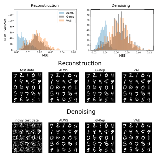
Top, mean squared error across 1,000 test inputs compared to G-Rep and VAE. Bottom, examples of real data, reconstructed and denoised samples.
Surprising findings: the vanilla VAE just failed on continuous and Fashion MNIST.
As mentioned in the beginning, we set out to train a generative model to generate fancy samples. However, we didn’t quite make that for large images such as CIFAR-10 or CelebA. Possible reasons are discussed in the paper.
However, we found that while our method achieves similar FID and KID scores on binary MNIST dataset with other maximum-likelihood-based methods (vanilla VAE, VAE with normalising flow posteriors and reweighted wake-sleep), it also win substantially on continuous MNIST and Fashion MNIST. In fact, on these datasets, our method is the only one that quickly finds a good solution while the other methods produced very strange behaviour shown in the figure below – the sample quality worsens with training.
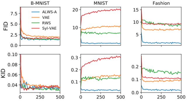
The horizontal axis is the number of epochs. Although ALWS is much slower compared with other methods, but the substantial advantage in sample quality is worth the cost.
This finding begs the question of whether it is meaningful to fight for and judge models based on log-likelihoods using binary MNIST dataset. Understandably, binary MNIST is simple, and estimating the log-likelihood using sampling methods (AIS) may be accurate. However, the bias in the normaliser depends on each model differently, and the decay of bias as a function of the samples can be very slow. From this finding, a good log-likelihood on binary MNIST does not necessarily mean the model behaves well for even the most closely-related datasets (at least all called MNIST).
But there should be no free lunch!
The no free lunch here is that we had to find the gradient model for every iteration. Since we used the consistent but notoriously slow kernel regression, each iteration takes quite a long time. It would be much more efficient if there is a way to train the gradient model incrementally but much more efficiently (like the recognition model in amortised inference). We discussed some other types of gradient models in the paper, and we hope to see more interesting ways to perform amortised learning!